Accuracy of atlc
In order to test the accuracy of atlc, some simple geometries were devised, for which there are known exact closed-form analytical solutions. The following have been tested. To date, all tests have yielded acceptable accuracy. Out of 48 tests, the higest error measured is 3.05%, with However, note that in most cases where the error is over 1%, is is clearly very obvious why it is. The conclusions at the end explain the reason for the higher errors observered on some simulations.
- Two_conductor_uniform_dielectricTwo-conductor transmission lines, with a uniform dielectric are discussed in section 1.0. Three cases were considered - the standard coaxial cable, an off-centre or eccentric coaxial cable and a symmetrical strip transmission line. These cases were consided since there are closed form exact analytical solutions on which to compare the results of atlc. Other structures will be tested at a later date.
- Two conductor transmission lines,
with two different dielectrics are described in section 2.
The only structure considered has been a dual coaxial cable, which has an inner and outer conductor like normal coaxiale cable, but has two different concentric dielectrics. This has an exact closed-form analytical solution. Testing a coaxial cable with thress or more multiple concentric dielectrics will later be performed, as it should be possible to derive an analytical formula for such a strucutre, although this has not currently be done.
I'm unaware of any other structure which has an exact solution when there are two or more dielectrics. If you know of any, please e-mail the details.
- Three conductors (directional coupler), with a single dielectric are described in section 3.0. For three-wires, which can be used to make a 4-port directional coupler, the accuracy was compared using two edge-on strip lines., as that is the only case I am aware of that has an exact analytical solution. However, comparisions with commercial tools such as the expensive HFSS package will be done at a later date. However, I am relieant on the help of others for this, since I don't personally have access to such expensive commerical software.
This section describes several tests for atlc using just two conductors and one dielectric. Several geometries have exact results, so it makes testing relatively easy.
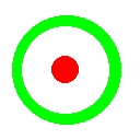 An obvious structure to test atlc with two conductor and a single dielectric is the round coaxial cable, which has an impedance:
Zo=59.95849160*loge(D/d)/sqrt(Er) Ohms
where D is the inner diameter of the outer conductor and d is the outer diameter of the inner conductor. (The number 59.958491602 is usually seen as 60 in most books, but that is only an approximation).
Circular conductors can never be defined exactly using a square grid, so differences between the exact answer and atlc's answer are due to:
- Errors in representing a circle on a square grid
- Errors in the method
atlc uses.
Seven coaxial cables were defined, which exibited a range of impedances between 5.5 and 179.6 Ohms. All eccept one used a vacuum dielectric. The table below shows the theoetical results and the results computed by atlc.
| Filename |
D |
d |
Er |
Zo (theory) |
Zo (atlc) |
Error (%) |
| coax-500-200-Er=100.bmp |
500 |
200 |
100.0 |
5.494 |
5.492 |
-0.036 % |
0m:43s |
| coax-500-400.bmp |
500 |
400 |
1.0 |
13.379 |
13.381 |
+ 0.020 % |
0m:11s |
| coax-500-200.bmp |
500 |
200 |
1.0 |
54.939 |
54.919 |
-0.036 % |
0m:43s |
| coax-400-82.bmp |
400 |
82 |
1.0 |
95.019 |
95.023 |
+0.004 % |
0m:31s |
| coax-500-100.bmp |
500 |
100 |
1.0 |
96.499 |
96.448 |
-0.053 % |
1m:08s |
| coax-500-50.bmp |
500 |
50 |
1.0 |
138.060 |
137.944 |
-0.008 % |
1m:22s |
| coax-500-25.bmp |
500 |
25 |
1.0 |
179.620 |
180.022 |
+0.244 % |
1m:28s |
Notes:
- These results were obtained with version 4.6.0 of atlc. Other versions will undoubtablly differ slightly as effort is made to improve the algorithms in atlc.
- Run times quoted are for a Sun Ultra 80 with 4 x 450 MHz and 4 Gb RAM, running Solaris 9. The compiler was gcc-3.2.2 with compiler options
-O2 -g.
- The only option used on atlc was the -d option on the occasions where the permittivity was not one of atlc's known values, so it needed to be specified on the command line
-
The largest error for the coaxial cables is only 0.244 %, the mean error is 0.017 % with the RMS error being 0.089 %.
- The larger error in the last result is due to the difficulty in accurately representing a small conductor on a reasonable sized grid. The ratio between the diameters of the outer and inner conductors is 20:1, making it difficult to represent both accurately without a grid become huge and so taking a lot of CPU time.
-
In some situations, accuracy can be improved at the expense of memory and CPU time, by using a finer grid and altering the cutoff parameter of atlc.
- As from version 4.6.0 of atlc, a new program called coax has been provided. This allows the quick computation of the impedance of a coaxial cable. To find the impedance of a coax with an inner of 32 mm, and outer of 120 mm and a relative permittivity of 2.2, just run coax:
% coax 32 120 2.2
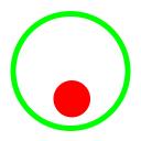
According to the book Microwave and Optical Components, Volume 1, - Microwave Passive and Antenna Components, page 7, there is an exact formula for the impedance of a coaxial line (see below). If O is the offset between the centres of the two conductors, then the impedance Zo assuming Er=1, is given by the following equation.
60 loge(x+sqrt(x^2-1)) where x=(d2+D2-4 O2)/(2*D*d)
This will allow a second check of atlc's accuracy with two conductors and one dielectric. Any problems which might be masked by the symmetry of the stardard coaxial cable will be eliminated.
Whenever the number 60 appears in formula for transmission lines, it should in fact be replaced by the number 59.9585. 60 is just a good approximation, but since we are testing atlc, the following formula will be used:
59.9585 loge(x+sqrt(x^2-1)) /sqrt(Er) where x=(d2+D2-4 O2)/(2*D*d)
Of course, one could constuct the a number of such transmission lines with a graphics package using its ability to draw circles, but getting the correct diamters and offsets would be time confusming. For this reasons the program create_bmp_for_circ_in_circ was used to generate a number of bitamps quickly with the following diameters and offsets.
| Filename |
D |
d |
O |
Er |
Zo (theory) |
Zo (atlc) |
Error (%) |
| eccentric-a.bmp |
500 |
400 |
40 |
2.15 |
5.482 |
5.487 |
+0.091 % |
| eccentric-b.bmp |
400 |
320 |
0 |
1.0 |
13.379 |
13.389 |
+0.075 % |
| eccentric-c.bmp |
500 |
100 |
100 |
10.0 |
29.707 |
29.713 |
+0.020 % |
| eccentric-d.bmp |
500 |
200 |
100 |
1.0 |
41.560 |
41.587 |
+0.065 % |
| eccentric-e.bmp |
500 |
200 |
10 |
1.0 |
54.825 |
54.862 |
+0.067 % |
| eccentric-f.bmp |
400 |
160 |
0 |
1.0 |
54.939 |
54.976 |
+0.067 % |
| eccentric-g.bmp |
400 |
40 |
12 |
5.0 |
61.644 |
61.676 |
+0.052 % |
| eccentric-h.bmp |
400 |
40 |
160 |
1.0 |
73.489 |
73.330 |
-0.216% |
| eccentric-i.bmp |
1600 |
160 |
640 |
1.0 |
73.489 |
73.330 |
-0.216 % |
| eccentric-j.bmp |
500 |
100 |
50 |
1.0 |
93.943 |
93.961 |
+0.019 % |
| eccentric-k.bmp |
500 |
100 |
0 |
1.0 |
96.499 |
96.524 |
+0.019 % |
| eccentric-l.bmp |
500 |
50 |
100 |
1.0 |
127.467 |
127.524 |
+0.045 % |
| eccentric-m.bmp |
500 |
50 |
50 |
1.0 |
135.586 |
135.654 |
+0.050 % |
| eccentric-n.bmp |
400 |
40 |
20 |
1.0 |
137.451 |
137.519 |
+0.049 % |
- These results were produced with version 4.6.0 of atlc. Results from other versions will probably differ, as efforts are made to further improve atlc.
- Due to their large size, the eccentric-?.bmp coax files are not distributed, but you could make them and compute their impedances like this. Add the -v option to create_bmp_for_circ_in_circ (as in example eccentric-d.bmp) if you want the theoretical results printed.
create_bmp_for_circ_in_circ 500 400 40 2.2 eccentric-a.bmp && atlc -d caff00=2.15 eccentric-a.bmp
create_bmp_for_circ_in_circ 400 320 0 1 eccentric-b.bmp && atlc eccentric-b.bmp
create_bmp_for_circ_in_circ 500 100 100 10 eccentric-c.bmp && atlc -d caff00=10 eccentric-c.bmp
create_bmp_for_circ_in_circ -v 500 200 100 1 eccentric-d.bmp && atlc
create_bmp_for_circ_in_circ 500 200 10 1 eccentric-e.bmp && atlc
create_bmp_for_circ_in_circ 400 160 0 1 eccentric-f.bmp && atlc
create_bmp_for_circ_in_circ 400 40 12 5 eccentric-g.bmp && atlc -d caff00=5 eccentric-g.bmp
create_bmp_for_circ_in_circ 400 400 160 1 eccentric-h.bmp && atlc
etc.
- If you add the
-v option to create_bmp_for_circ_in_circ, it will print the exact theoretical values for you too.
- If you only want to compute the impedance of an offset coax, without actually creating the bitmap, the program coax can be used, if you supply the
-o offset option. For example:
coax -o 40 400 500 1
Zo =         8.038255 Ohms
- Since there is an exact answer to this geometry, even when the inner is offset, there is not a lot of point in spending seconds or minutes running
atlc to come an approximate numerical answer, when you can compute an exact one in a small fraction of a second. However, using atlc to compute a few of these gives you confidence atlc is working properly.
Another obvious test to determine the performance of atlc with two conductors and one dielectric is a symmetrical strip transmission line - see diagramme below.

This has an exact analytical solution, dependent on the ratio of the
width of the inner conductor w, to the distance between the two outer
conductors H. This assumes that the outer conductors extend to plus
and minus infinity and the inner conductor is infinitely thin. This
structure has the advantage of requiring no curves, so can be
represented accurately with the square grid used in atlc.
However, its impossible to have an inner conductor that is less than 1 pixel
high and it is impossible to make the dimension W infinitely wide as it
was take an infinite amount of disk space, RAM and CPU time. However, if
the width W is made at least 4xH+w, then making it any larger does not
seem to have much affect on the result.
The -i option to create_bmp_for_symmetrical_stripline,
forces the width
W to be equal to 4 times the internal height plus the inner conductor's
width w (unless the user specified a larger value of W). Hence, when
the -i option is used, a valid test of atlc's
accuracy can be made
Without the -i option, you can made the width W and height
H any value
you want above >=5 pixels, although H must be odd, for the inner conductor
to fit equally between the two outer confuctors. As always, the bitmaps created
are 10 pixels higher and 10 pixels wider, to enforce a green metallic boundary that is cleraly visable.
create_bmp_for_symmetrical_stripline -vv -i 0 201 290 50-201.bmp


For this to be a valid test of atlc, the width should be

infinite. Since you used the -i option (indicationg you

want the width W to effectively infinite, W must exceed w + 4xH.

Therefore W has been is set to 1134

w=290 H=201 w/H=1.442786 xo=23.7538

Zo is theoretically 49.989477 Ohms (assuming W is infinite)
This structure, which has a w/H value of 1.442786, has a theoretical impedance close to 50 Ohms (49.989477 to be precise). Version 4.6.0 of atlc calculates this to be 49.899 Ohms, an error of -0.181%, when using a grid 1134x201.
| Filename |
W |
H |
w |
w/H |
Zoexact |
Zoatlc |
Error |
Time |
| 25ohm-201h.bmp |
1512 |
201 |
668 |
3.3234 |
25.018 |
24.932 |
-0.344 % |
0h:00m:46s |
| 25ohm-401h.bmp |
2978 |
401 |
1334 |
3.3267 |
24.996 |
24.940 |
-0.224% |
0h:08m:52s |
| 25ohm-801h.bmp |
6000 |
801 |
2664 |
3.3267 |
25.001 |
24.935 |
-0.264% |
1h:49m:46s |
| 50ohm-201h.bmp |
1134 |
201 |
290 |
1.42786 |
49.989 |
49.899 |
-0.180% |
0h:00m:37s |
| 50ohm-401h.bmp |
2222 |
401 |
578 |
1.4419 |
50.026 |
49.944 |
-0.164% |
0h:07m:16s |
| 50ohm-801h.bmp |
4399 |
801 |
1155 |
1.4419 |
50.012 |
49.878 |
-0.268% |
1h:46m:31 |
| 100ohm-201h.bmp |
945 |
201 |
101 |
0.5025 |
100.161 |
100.319 |
+0.158% |
0h:00m:34s |
| 100ohm-401h.bmp |
1846 |
401 |
202 |
0.5037 |
100.02 |
99.998 |
-0.022% |
0h:06m:42s |
| 100ohm-801h.bmp |
3647 |
801 |
403 |
0.5037 |
100.09 |
99.857 |
-0.233% |
1h:29m:17s |
| 200ohm-201h.bmp |
862 |
201 |
18 |
0.0896 |
200.81 |
204.210 |
+1.693% |
0h:0m:31s |
| 200ohm-401h.bmp |
1680 |
401 |
36 |
0.08978 |
200.669 |
201.844 |
+0.586% |
0h:06m:22s |
| 200ohm-801h |
3317 |
801 |
73 |
0.09114 |
199.771 |
199.734 |
-0.019% |
1h:23m:08s |
| 400ohm-1551h |
6439 |
1551 |
5 |
0.00322 |
400.040 |
417.700 |
+4.415% |
12h:20m:50s |
| 400ohm-76610h |
31109 |
7750 |
25 |
0.00323 |
400.085 |
|
% |
|
Notes:
- These results were produced with version 4.6.0 of atlc. Results from other versions will probably differ, as efforts are made to further improve atlc.
- For the same sepparation between the two outer conductors h, the width of the inner conductor w decreases as the impedance of the line is increased. When this width w is too small, accuracy suffers. In order to get reasonable accuracy it is essential to use sufficient pixels for the width of the conductor w.
- Run times are given when compiled single-threaded, with
gcc-3.2.2 on a Sun Ultra 80 workstation with 4x450 MHz CPUs and 4 GB of RAM. Compiler options of -O2 -g were used. - Only 1 CPU in the Ultra 80 would have been used, since
atlc
was compiled single-threaded.
-
The -s and -S options were given to
atlc so that it did
not create bitmap files. Without these options, run times would be a
little longer, due to the time to write the files to disk.
- Compiled as a multi-threaded application to use all 4 CPUs in a Sun
Ultra 80, the run times reduce by a factor of approximately 3.5.
- The result for the first 400 Ohm transmission line analysed (400ohm-1551h.bmp) is very poor (3.5% error)
since only 5 pixels could be used for the width of the inner conductor.
The results from this test are not included when calculating the overall
accuracy of atlc, since using only 5 pixels is not a fair test.
An attempt at using 25 pixels for the inner conductor's width, where accuracy should
have been better, created a 689 MB bitmap file, which could not be analysed, as
the RAM in the computer (2 GB) was insufficient, although this might be tried later since the computer has since been upgraded.
Section 2. Two-conductor Transmission Lines with a non-uniform dielectric
Destermining altc's accurarcy with multiple-dielectrics is not easy, as there are few analytical methods. The only one known in dual dielectric coax. At a later date some comparisions will be made to commerical software if this is possible.
2.1 Comparision of atlc and a dual dielectric coaxial cable
A coaxial cable with two concentric dielectrics like that below

has an exact analytical solution. The red is the inner conductor, the green forms the outer conductor. The light blue and orange regions are both dielectrics, neither of which are one of atlc's predefined colours, so the dielectric constant of both must be set by issuing the -d option to atlc. (The light blue in this image, is not to be confused with the light blue that is pre-defined for PTFE with a dielectric constant of 2.1).
A small program called dualcoax can be used to compute the impedance of a dual coaxial cable. If the diameter of the inner conductor is 135, the inner dielectric 337, the internal diameter of the outer conductor is 401, the permittivity of the inner dielectric 2.0 and the outer dielectric 3.0, then:
$ dualcoax 135 337 401 2.0 3.0
will compute the impedance, which is 44.912 Ohms.
The following table shows the impedances for various values of permittivity of both the inner and outer dielectrics. Note that changing the relative permittivity of the outer conductor has little effect, as it is quite thin, whereas the outer dielectric is much thicker and so has more effect on the impedance.
| Filename |
D1 |
D2 |
D3 |
Erinner |
Erouter |
Zo(theory) |
Zo(atlc) |
Error |
Time |
| dual-dielectric-coax.bmp |
156 |
400 |
500 |
1.0 |
1.0 |
69.837 |
69.848 |
+0.017% |
0h:00m:59s |
| dual-dielectric-coax.bmp |
156 |
400 |
500 |
3.0 |
1.0 |
47.420 |
46.681 |
-1.559% |
0h:04m:35s |
| dual-dielectric-coax.bmp |
156 |
400 |
500 |
10.0 |
1.0 |
36.451 |
35.839 |
-1.679 % |
0h:10m:17s |
| dual-dielectric-coax.bmp |
156 |
400 |
500 |
30.0 |
1.0 |
32.647 |
32.314 |
-1.020% |
0h:17m:53s |
| dual-dielectric-coax.bmp |
156 |
400 |
500 |
1000000.0 |
1.0 |
30.568 |
30.330 |
-0.779 % |
1h:18m:17s |
| dual-dielectric-coax.bmp |
156 |
400 |
500 |
1.0 |
2.0 |
66.408 |
65.974 |
+0.658% |
0h:02m:01s |
| dual-dielectric-coax.bmp |
156 |
400 |
500 |
1.0 |
1000000.0 |
62.792 |
62.727 |
-0.014% |
0h:10m:02s |
| dual-dielectric-coax.bmp |
156 |
400 |
500 |
2.5 |
3.5 |
42.943 |
42.858 |
-0.198 % |
0h:01m:55s |
Notes:
- These results were produced with version 4.6.0 of
atlc.
-
To compute these results, one must run atlc with the -d option to define what the relative dielectric constant for each colour, as described in the section on producing suitable bitmaps. The light blue colour has a hex representation of 0x8b8dff and the orange is 0xfd8a11. So for the last entry in the table, one would run
$ atlc -d fd8a11=2.5 -d 8b8dff=3.5 dual-dielectric-coax.bmp
Ckearly the accuracy of atlc with multiple dielectrics is lower than that with a single dielectric, where typical errors are around 0.1%. This is believed to be due to the fact the equations used when there are multiple dielectrics are not precise and in a later version it is hoped to refine the equations, so accuracy improves.
Testing the accuracy of atlc with coupled lines is more difficult that with single isolated lines, since there is to my knowledge only one structure for which exact analytical results exist. For two infinitely thin conductors halfway between two infinitely wide groundplanes (see below)

the odd and even mode impedances can be calculated analytically. If the spacing between the two groundplanes is H, the width of the conductors w, the spacing between the conductors s, and the permittivity of the medium Er,
----------^--------------------------------------------------------------
          |
          |                <---w---><-----s----><---w-->
          H                ---------            --------
          |       Er
          |
----------v--------------------------------------------------------------
then, according to the book by Matthaei, Young and Jones called Microwave Filters, Impedance Matching Networks and Coupling Structures, Artech House, Dedham, MA., 1980. the impedances are given by
Zeven=(30*pi/sqrt(er))*(K(ke')/K(ke))
Zodd=(30*pi/sqrt(er))*(K(ko')/K(ko))
K(kx)=complete elliptic integral of the first kind.
ke=(tanh((pi/2)*(w/H)))*tanh((pi/2)*(w+s)/H)
ko=(tanh((pi/2)*(w/H)))*coth((pi/2)*(w+s)/H)
ke'=sqrt(1-(ke^2))
ko'=sqrt(1-(ko^2))
Again, I suspect 30 is just an approximation, like 60 is used in the impedance for coax, and so the values should be:
Zeven=(29.97924580*pi/sqrt(er))*(K(ke')/K(ke))
Zodd=(29.97924580*pi/sqrt(er))*(K(ko')/K(ko))
I'm very grateful to Paul Gili AA1LL / KB1CZP aa1l@email.com for providing me with these equations, references and nomographs.
A programme create_bmp_for_stripline_coupler was written to automatically generate bitmaps given the height H between the groundplanes, the conductor widths w and spacing s. Ideally this needs simulating from -infinity to +infinity, but that is not practical. It was assumed that if the complete structure width W was equal to 2*w+s+8*H that would be adequate (this seemed about right, but I've no proof it is optimal). As well as producing a bitmap, create_bmp_for_stripline_coupleralso calculates the theoretical values of impedance.
The above were created using the following set of commands
$ create_bmp_for_stripline_coupler -v 1 1 1 1 coupler1.bmp
$ create_bmp_for_stripline_coupler -v 1.991 1 1 1 coupler2.bmp
$ create_bmp_for_stripline_coupler -v 3 1 1 1 coupler3.bmp
$ create_bmp_for_stripline_coupler -v 5 1 1 1 coupler4.bmp
$ create_bmp_for_stripline_coupler -v 1 1 0.5 1 coupler5.bmp
$ create_bmp_for_stripline_coupler -v 1 1 0.099 1 coupler6.bmp
$ create_bmp_for_stripline_coupler -v 0.25 1.19 1.34 2.2 coupler7.bmp
| Filename |
H |
w |
s |
Er |
Zoddtheory |
Zoddatlc |
Errorodd |
Zeventheory |
Zevenatlc |
Erroreven |
| coupler1.bmp |
1.0 |
1.0 |
1.0 |
1.0 |
64.723 |
64.308 |
-0.641% |
65.969 |
65.540 |
-0.300% |
| coupler2.bmp |
1.991 |
1.0 |
1.0 |
1.0 |
93.056 |
92.711 |
-0.371% |
106.830 |
106.437 |
-0.368% |
| coupler3.bmp |
3.0 |
1.0 |
1.0 |
1.0 |
105.409 |
105.072 |
-0.320% |
139.670 |
139.091 |
-0.415% |
| coupler4.bmp |
5.0 |
1.0 |
1.0 |
1.0 |
114.237 |
114.217 |
-0.018% |
189.135 |
188.629 |
-0.268% |
| coupler5.bmp |
1.0 |
1.0 |
0.5 |
1.0 |
62.133 |
61.887 |
-0.396% |
68.215 |
67.941 |
-0.402% |
| coupler6.bmp |
1.0 |
1.0 |
.099 |
1.0 |
50.614 |
50.546 |
-0.134% |
74.377 |
73.883 |
-0.664% |
| coupler7.bmp |
0.25 |
1.19 |
1.34 |
2.2 |
12.208 |
12.062 |
-1.196% |
12.208 |
12.062 |
-1.196% |
Note:
- The data was collected with version 4.6.0 of atlc. As always, the data may change with later versions of atlc, as the code is further improved.
- The theoretical impedance quoted are for the dimensions in the table. The actual bitmap produced will frequently not be the same as it's impossible to represent perfectly an arbitrary grid on a grid with finite resolution. The program
create_bmp_for_stripline_coupler also computes the theoretical valus for the actual grid generated, but these have not been used.
- There seems to be some systematic error for this coupler, as the impedances determined by atlc are always below the theoretical values. The source of this error will be investigated. It is clear that the error decreases as the height h is increased.
- Run times quoted are for a Sun Ultra 80 with 4 x 450 MHz and 4 Gb RAM, running Solaris 9. The compiler was gcc-3.2.2 with compiler options
-O2 -g.
Section 4. Conclusions about the accuracy of atlc
Looking at the above data it is clear that on some structures (such as a standard coaxial cable or an eccentric cable, the accuracy of atlc is excellent. Of the 21 tests for these structures, 18 had errors of below 0.1% and the other three had errors below 0.25%. Each structure is round, with a minimum diamater of 25 pixels. The outside edge has around Pi*25=79 pixels to reprsent it, so errors due to quantising the electric field are quite small.
Of the three results for coaxial and eccentric cables that show errors over 0.1%, the reasons are not had to understand. File coax-500-25.bmp has the smallest number of pixels for the centre conductor in any of the standard coaxial cables. With the smallest number of pixels (a diameter of 25 and a circumference of 78 pixels), the errors can be expected to be highest. It is likely the errors could be reduced by making conductors larger, but there is no point, as the error (just 0.244%) are negligable.
You can't expect to accurately model any structure where one of the critical dimensions is represented by too few pixels.
Clearly if any dimention needs to be reprsented by 5.4 pizels, the nearest number is 5 pixels, so immediately an error of 8% has been introduced. But since the electric field (which varies continuously) is only computed at 5 places, the true varition can't be known accurately.
As a rule of thumb, try to keep any critital dimension to at least 25 pixels.
Return to the atlc homepage
atlc is written and supported by Dr. David Kirkby (G8WRB) It it issued under the GNU General Public License


The following is a trap for smammers, so they can gather loads of ficticious email address, so don't click anywhere
o
n
this
line
th
anks.